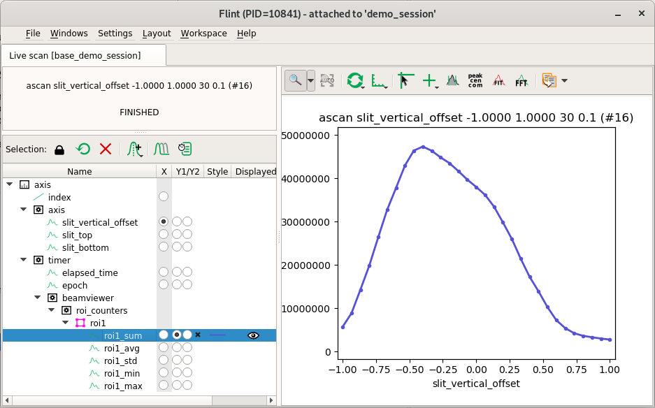
Live curve

If the scan contains counters, the curve widget will be displayed automatically.

Compare scans

A tool provided in the property tool bar allow to compare scans.

When activated is allows to stack new coming scans.

The channel selection will be displayed for the whole scans.

If the scan to compare with is still in the Redis history, it can be loaded with the dedicated tool from the property tool bar.

APIs

Here is the available commands which can be used from the BLISS shell.

Get the plot

Here is a way to access to a curve plot from BLISS.

f = flint()

scan = ascan(sx,0,2,100,0.01, diode1, diode2)

# Make sure flint is up to date with the last scan
f.wait_end_of_scans()

# Get the live plot
p = f.get_live_plot("default-curve")

Interactive data selection

This plot provides an API to interact with region of interest.

Axis scale

# Change the axis scale
p.yscale = "log"  # Or "linear"

User data

The following lines shows how to add processed data from BLISS shell.

scan = ascan(sx,0,2,100,0.01, diode1, diode2)

# Denoise the signal from the diode1
import scipy.signal
ydata = scan.get_data()[diode1.fullname]
n = 15
b = [1.0 / n] * n
ydenoised = scipy.signal.lfilter(b, 1, ydata)

# Make sure flint is uptodate with the last scan
f.wait_end_of_scans()

# Get the live plot and attach the denoised signal to the diode1
p = f.get_live_plot("default-curve")
p.update_user_data("denoized", diode1.fullname, ydenoised)

Axis markers

Code example to add a marker (vertical line) on a curve.

A marker is relative to an axis. Here mm2 is expected, and the marker will only be displayed if this axis is the actual one used in the plot.

ascan(mm2, 3.14, 7.28, 5, 0.1, savoie)
p = flint().get_live_plot("default-curve")
p.update_axis_marker("mark5d", "axis:mm2", 5.01, "bla bla")