Flint, online data visualisation tool
What is Flint
- Flint is not silx-view
- Flint is not PyMca
- Flint is meant to replace the Spec GUI and Oxidis
Flint is a GUI intending to display raw data generated by BLISS, mostly to help beamline alignment.
It also provides graphic interaction for user scripts.
Demo session
The BLISS demo session can be used as a show case for Flint.
Make sure all demo servers are started.
Starting Flint
If the session is configured for it (which is the case for the demo session), Flint will be started by the call to any standard scan command.
It can be enabled this way:
SCAN_DISPLAY.auto = True
Overview
The demo session provides simulated slits coupled with a camera already setup with a ROI.
We can open the slits and scan the beam this way:
mv(slit_vertical_gap, 1)
ascan(slit_vertical_offset, -5.0, 5.0, 20, 0.1, beamviewer.roi_counters)
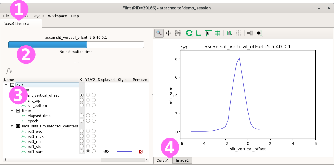
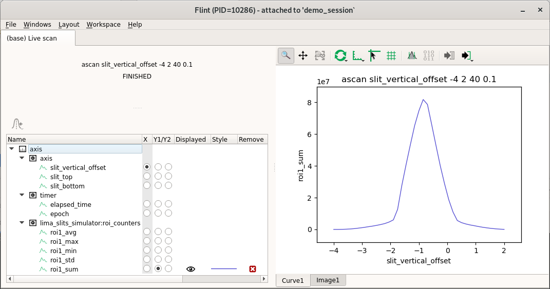
Flint provides a ➊ Live screen containing various widgets.
A widget ➋ provides the current scan progress, a ➌ property widget to customize the content of the plots, and ➍ the following are provided to display scan data.
Curve
The previous scan displays the following result.
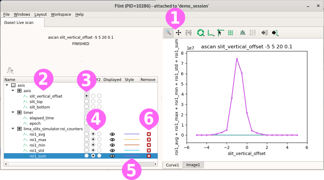
The curve widget provides a ➊ toolbar to interact with the plot. It contains tools to:
- zoom and pan the view
- customize the refresh rate of the data
- change the axes’ configuration
- plus other specific actions
The property view provides tools to customise items displayed by the plot. Items are identified by their ➋ names (usually the name of the counter), the ➌ x-axis can be selected, the data can be ➍ displayed using the left or right y-axis.
Curve styles ➎ are automatically selected depending on the content of the scan. These styles cannot be customized.
Items can be ➏ removed from the plot. A removed item is still available and can be re-displayed. However, no style is assigned to it.
Manual selection
The curve widget can be configured to display or hide the data obtained during the scan.
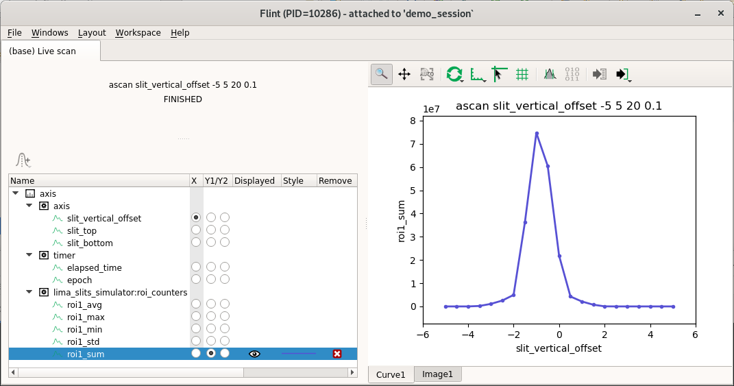
As long as the same devices are scanned, this setup will be reused unchanged (technically speaking, while the acquisition chain is the same as used for the displayed scan previously).
Refinment of the scan
The scan values, like the motor range or the number of points, can be tuned, without losing the custom selection.
ascan(slit_vertical_offset, -4.0, 2.0, 40, 0.1, beamviewer.roi_counters)
Gaussian, derivative, and markers
Several tools are provided to annotate the displayed curves in Flint.
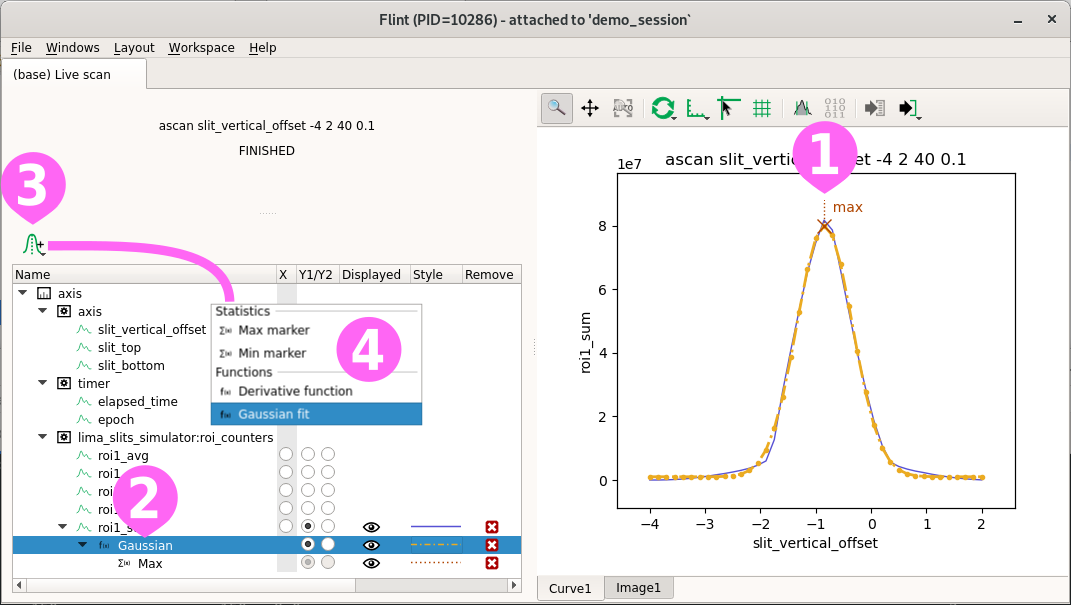
Computed items ➊➋ can be created based on a selected curve. The result can be displayed after data processing of choice.
A tool ➌ is provided to create computed markers or apply functions to the selected curve. It provides ➍ a few features, like markers for the location of maximum or minimum, a gaussian fit or a derivative function.
As for curve selection, this information will only persist while the acquisition chain remains unchanged.
Command-line selection
BLISS offers two ways to select a specific curve.
plotselect chooses the counters to be displayed. It can be used any time and even changes a plot on display. The same can be done with the mouse.
ascan(slit_vertical_offset, -4.0, 2.0, 40, 0.1, beamviewer.roi_counters)

...

plotselect("beamviewer:roi_counters:roi1_avg")
plotinit can be used before an acquisition and remains valid only for this next scan. It selects the counters to be displayed when reading back a scan from the database (redis). All counters will be acquired and stored.
plotinit("beamviewer:roi_counters:roi1_avg")
ascan(slit_vertical_offset, -4.0, 2.0, 40, 0.1, beamviewer.roi_counters)
Scatters
The demo session provides a simulation diode connected to sy and sz motors.
This can be used to do meshes.
amesh(sy, -.75, .75, 30, sz, -.75, .75, 30, .001, fluo_diode)
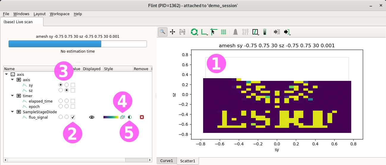
The default plot for meshes uses a ➊ scatter plot, with an image based rendering.
The property widget allows to ➋ select the main diode to display and to choose the ➌ axes. It also provides a dialog for ➍ custom rendering and ➎ editing colormap and brightness.
Other ➍ renderings are provided, like point based -, or solid interpolation. Flint also supports fixed rendering. For example, points can be displayed on top of a solid rendering,
Scatters with motor displacement
The demo session provides motor encoders configured to follow sy and sz and
offers noise as a signal. This can be used to simulate scans.
amesh(sy, -.1, .1, 20, sz, -.3, .3, 30, .001, fluo_diode,
                                              sy.encoder,
                                              sz.encoder)
Instead of the motors, the encoders can be selected as axes.
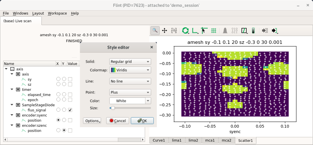
The regular grid mode is based on an image, and is then very fast to render. An overlay with the location of the points can be added to check the displacements.
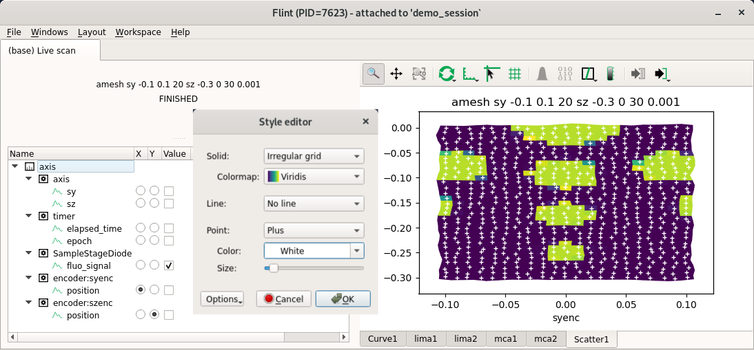
The irregular grid mode is based on mesh computed around the mesured points. This rendering is much slower without OpenGL, but can help to notice bigger displacements. The points can also be overlayed.
Curves from scatter data
Curve widgets can also be used to display grids.
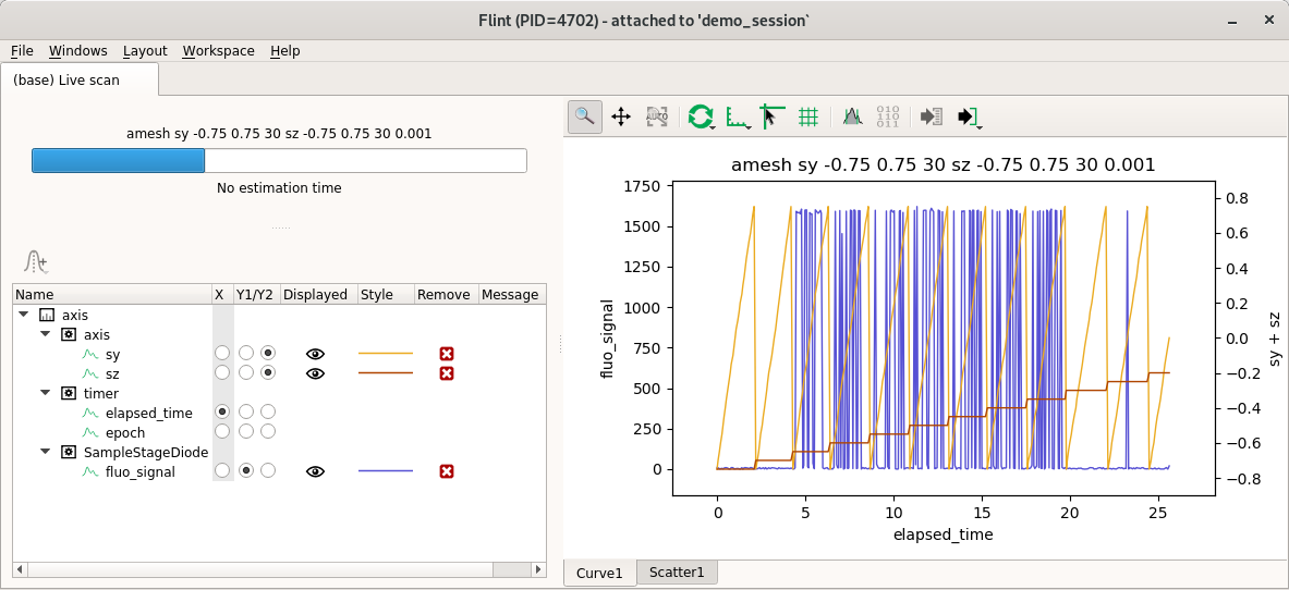
They present the values of data acquisition over time.
MCAs
Flint provides a basic view of MCA spectra.
A single scan can involve many spectra. Usually one would use a single and always the same widget for each detector.
timescan(1, tomocam)
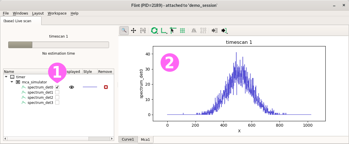
The configuration dialog ➊ allows to select one or several spectra to display.
For now, only raw spectra ➋ (count per channels) are displayed.
More features, like plots in energy, could be provided, but Flint should not replace pymca.
Images
Flint supports image (2d) display.
A single scan can contain many spectra. Usually one would use a single and always the same widget for each detector.
The demo session provides a tomography projection example.
timescan(1, tomocam)
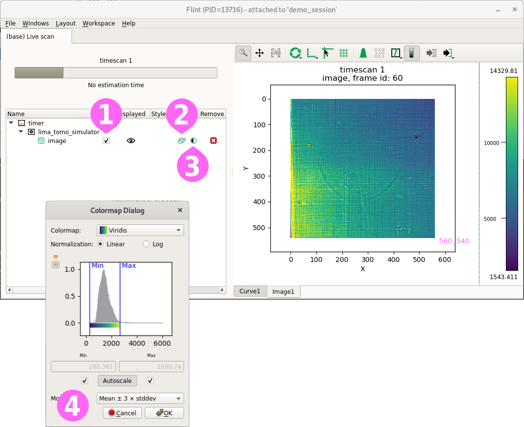
We can distinguish a diatom on a top of a needle.
The property widget ➊ allows to select one image if there are many. It also provides a dialog for ➋ custom rendering and ➌ editing colormap and brightness.
Editing Lima ROIs
Lima ROIs can be edited from within BLISS by way of the edit_roi_counters command. This command uses the Flint programming interface, which is available for user scripts.
edit_roi_counters(tomocam, 0.1)
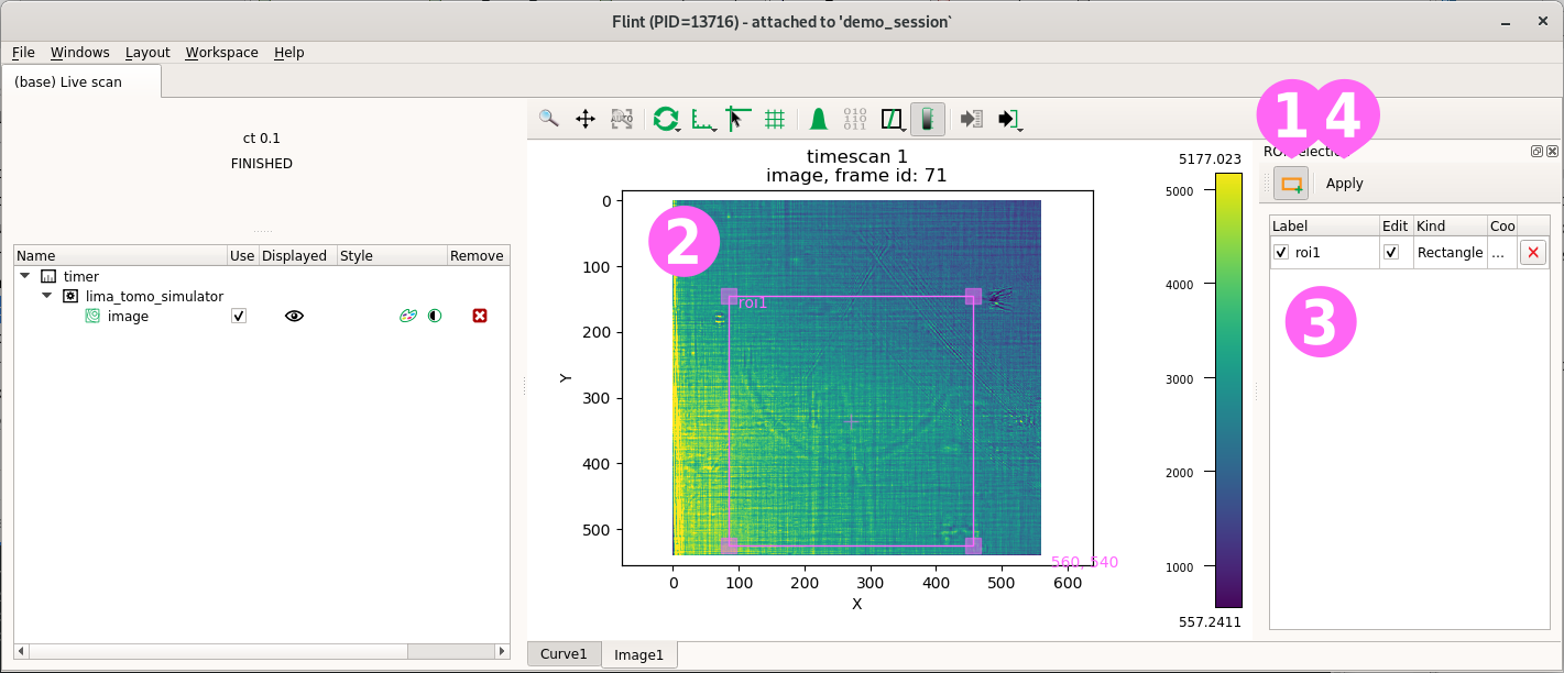
Switch the interaction to ‘ROI mode’ ➊. This allows to create ➋ new rectangular ROIs. A list of available ROIs ➌ is displayed and can be used to edit or remove ROIs. The Apply button ➍ is there to validate the choice.
When used from BLISS the selection can be cancelled using Ctrl-c.
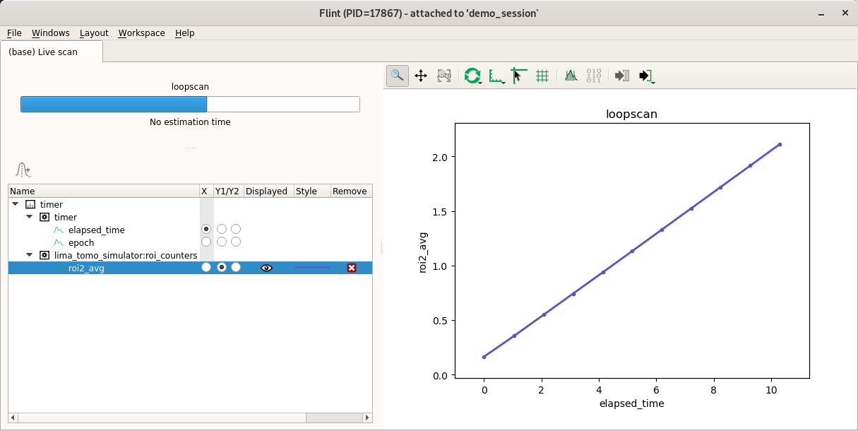
This ROIs can now be used in a scan.
loopscan(20, 1, tomocam.counters.roi2_avg)