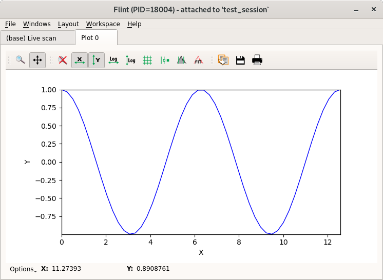
1D plot / curve plot
Viewer to display a set of curves.
It provides 2 ways to request a plot.
- Descriptive way (recommended)
- Imperative way
Descriptive way
The 1D plot provides a descriptive way to define the display.
It is the recommended way, because it splits the data and it’s representation.
This simplifies the upload of data, reuse some data instead of duplication, provides a better handling of the rendering. Plus this will provide more flexibility for the future.
The description have to be done it 2 steps
- The description of what to display (using string reference)
- The upload of the data
import numpy

# Create the plot
f = flint()
p = f.get_plot("curve", name="My plot")

# Create the data
t = numpy.linspace(0, 10 * numpy.pi, 100)
s1 = numpy.sin(t)
s2 = numpy.sin(t + numpy.pi * 0.5)
s3 = numpy.sin(t + numpy.pi * 1.0)
s4 = numpy.sin(t + numpy.pi * 1.5)

# Describe the plot
p.add_curve_item("t", "s1")
p.add_curve_item("t", "s2")
p.add_curve_item("t", "s3")
p.add_curve_item("t", "s4")

# Transfer the data / and update the plot
p.set_data(t=t, s1=s1, s2=s2, s3=s3, s4=s4)

# As the plot description is already known
# The plot can be updated the same way again
p.set_data(t=t+1, s1=s1+1, s2=s2+1, s3=s3+1, s4=s4+1)

# Clean up the plot
p.clean_data()
Imperative way
The imperative way allow you to tell what you want to display, instructions after instructions.
It is not recommended, because it will not allow you to handle properly the rendering, and as result will create blinking,
It is still supported for compatibility with old code.
import numpy

# Create the plot
f = flint()
p = f.get_plot("curve", name="My plot")

# Create data
t = numpy.linspace(0, 10 * numpy.pi, 100)
s = numpy.sin(t)
c = numpy.cos(t)

# Update the plot
p.add_curve(t, c, legend="aaa")  # the legend have to be unique
p.add_curve(t, s, legend="bbb")

# Clean up the plot
p.clean_data()
APIs
Axes label
Property are provided to tune the axes label.
p.xlabel = "It's the time"
Axes scale
Property are provided to tune the axes scale.
p.yscale = "log"
p.xscale = "linear"
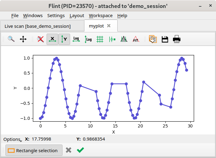
Curve edition
The helper select_points_to_remove can be used to remove points from a curve
plot item.
The UI allow to select points to remove. This interaction can be accepted with a validation button. Another button allow you to cancel the changes, as result the original curve is restored.
Here is an example to edit a single curve item.
If you have an items sharing the save x-axis, an extra parameter allow you to update extra data at the same time.
# Setup a sinusoid curve
import numpy
f = flint()
p = f.get_plot("curve", unique_name="myplot")
datax = numpy.linspace(0, 10 * numpy.pi, 100)
datay = numpy.sin(datax + numpy.pi * 1.5)
p.add_curve_item("x", "y", legend="myitem", linewidth=1)
p.set_data(x=datax, y=datay)

# Request the user to edit the curve
res = p.select_points_to_remove("myitem")

# Finally the edited result can be retrieved from the plot
if res:
    print("The curve was edited")
    x = p.get_data("x")
    y = p.get_data("y")
Transaction
For complex plot, if you want to handle properly the refresh of the plot a transaction can be used. It will enforce a single update of the plot at the end of the transaction.
with p.transaction():
    p.clear_items()
    p.add_curve_item("x", "y", legend="item1")
    p.add_curve_item("x", "w", legend="item2")
    p.remove_item(legend="item2")
    p.set_data(x=[1])
    p.append_data(x=[2, 3, 4, 5])
    p.set_data(y=[6, 5, 6, 5, 6])