Example of custom scan_info

This examples show how to describe metadata in scan_info for few specific scans.

The main use case is to: - Allow to display scatter as a solid regular 2D image. - Display the entire region of the scan before the end

Displaying scatter data as a scatter of points is not a problem.

With this extra metadata, the user can decide to use a solid or point based rendering.

Setup

This scans have to be created usually per beamline in a very specific way.

For this examples we will use a function to simulate them.

import gevent
import numpy
from bliss.scanning.group import Sequence
from bliss.scanning.chain import AcquisitionChannel

def simulate_scan(scan_info, data):
    """
    Simulate a scan.

    It uses a sequence to emit custom channels.

    Arguments:
        scan_info: Dictionary contanining metadata to store with the scan
        data: Dictionary containing numpy array per channel name
    """
    step = 2
    seq = Sequence(scan_info=scan_info)
    for channel_name, array in data.items():
        seq.add_custom_channel(AcquisitionChannel(channel_name, float, ()))
    with seq.sequence_context() as scan_seq:
        array = list(data.values())[0]
        for i in range(0, len(array) - 1, step):
            selection = slice(i, i + step)
            for channel_name, array in data.items():
                seq.custom_channels[channel_name].emit(array[selection])
            gevent.sleep(0.1)

Regular scatter

This example create a regular scatter.

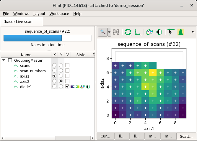
from bliss.scanning.scan_info import ScanInfo
import numpy

scan_info = ScanInfo()

# Specify the same group for all this channels (axis or values)
scan_info.set_channel_meta("axis1",
                           # The group have to be the same for all this channels
                           group="foo",
                           # This is the fast axis
                           axis_id=0,
                           # In forth direction only
                           axis_kind="forth",
                           # The grid have to be specified
                           start=0, stop=9, axis_points=10,
                           # Optionally the full number of points can be specified
                           points=100)
scan_info.set_channel_meta("axis2", group="foo", axis_id=1,
                           axis_kind="forth",
                           start=0, stop=9,
                           axis_points=10, points=100)
scan_info.set_channel_meta("diode1", group="foo")

# Request a specific scatter to be displayed
scan_info.add_scatter_plot(x="axis1", y="axis2", value="diode1")

# Generate the data
slow, fast = numpy.mgrid[0:10, 0:10]
dist = (((slow - 4.5) ** 2 + (fast - 4.5) ** 2) ** 0.5)
dist = (dist.max() - dist) * 10
data = {
    "axis1": fast.flatten(),
    "axis2": slow.flatten(),
    "diode1": numpy.random.poisson(dist.flatten())
}

SCAN_DISPLAY.auto = True
simulate_scan(scan_info, data)

Regular 3D scatter

3D of more dimensions are supported.

Flint only can display it using the 2 fastest axes.

Other axes have to be stepper and are considered as an ndim index for the displayed frame.

displayed.

For now only Flint will only display the last frame.

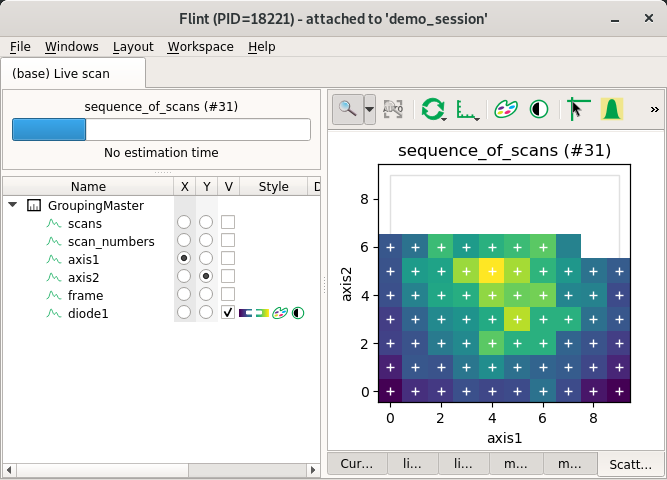
from bliss.scanning.scan_info import ScanInfo
import numpy

scan_info = ScanInfo()

scan_info.set_channel_meta("axis1", group="foo", axis_id=0,
                           axis_kind="forth",
                           start=0, stop=9, axis_points=10,
                           points=1000)
scan_info.set_channel_meta("axis2", group="foo", axis_id=1,
                           axis_kind="forth",
                           start=0, stop=9, axis_points=10,
                           points=1000)
# The slowest axes have to be describe as stepper
scan_info.set_channel_meta("frame", group="foo", axis_id=2,
                           axis_kind="step",
                           start=0, stop=9, axis_points=10,
                           points=1000)
scan_info.set_channel_meta("diode1", group="foo")

# Request a specific scatter to be displayed
scan_info.add_scatter_plot(x="axis1", y="axis2", value="diode1")

# Generate the data
frame, slow, fast = numpy.mgrid[0:10, 0:10, 0:10]
dist = (((slow - 4.5) ** 2 + (fast - 4.5) ** 2) ** 0.5)
dist = (dist.max() - dist) * 10
data = {
    "axis1": fast.flatten(),
    "axis2": slow.flatten(),
    "frame": frame.flatten(),
    "diode1": numpy.random.poisson(dist.flatten())
}

SCAN_DISPLAY.auto = True
simulate_scan(scan_info, data)

Theorical and encoder position together in scatter

The same axis can be describe many time using many channels.

That’s what we simulate here. axis1 and axis2 are also provided as axis1-enc, axis2-enc.

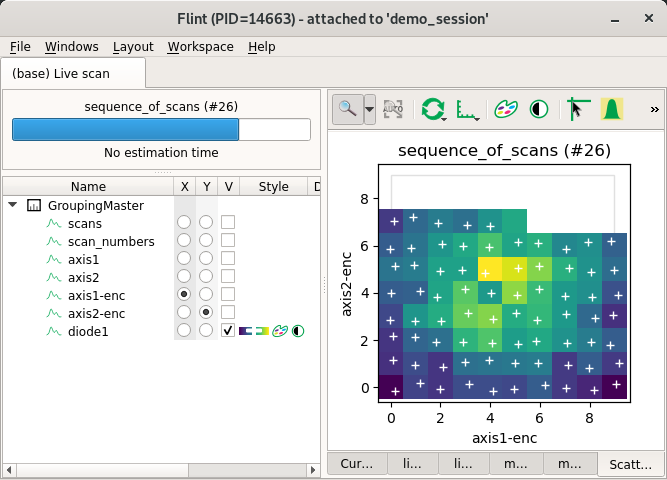
from bliss.scanning.scan_info import ScanInfo
import numpy

scan_info = ScanInfo()

scan_info.set_channel_meta("axis1", group="foo", axis_id=0, axis_kind="forth",
                           start=0, stop=9, axis_points=10, points=100)
scan_info.set_channel_meta("axis2", group="foo", axis_id=1, axis_kind="forth",
                           start=0, stop=9, axis_points=10, points=100)
# Index are reused for the encoded
scan_info.set_channel_meta("axis1-enc", group="foo", axis_id=0, axis_kind="forth",
                           start=0, stop=9, axis_points=10, points=100)
scan_info.set_channel_meta("axis2-enc", group="foo", axis_id=1, axis_kind="forth",
                           start=0, stop=9, axis_points=10, points=100)
scan_info.set_channel_meta("diode1", group="foo")

# Request a specific scatter to be displayed
scan_info.add_scatter_plot(x="axis1", y="axis2", value="diode1")

# Generate the data
slow, fast = numpy.mgrid[0:10, 0:10]
dist = (((slow - 4.5) ** 2 + (fast - 4.5) ** 2) ** 0.5)
dist = (dist.max() - dist) * 10
data = {
    "axis1": fast.flatten(),
    "axis2": slow.flatten(),
    "axis1-enc": fast.flatten() + (numpy.random.rand(100) * 0.4 - 0.2),
    "axis2-enc": slow.flatten() + (numpy.random.rand(100) * 0.4 - 0.2),
    "diode1": numpy.random.poisson(dist.flatten())
}

SCAN_DISPLAY.auto = True
simulate_scan(scan_info, data)

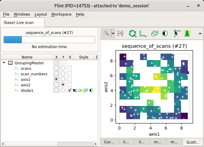
Back and forth axis scatter

For now Flint is not able to display it with a solid rendering. It could be displayed as a regular grid.

For now you can use metadata for non-regular scatters.

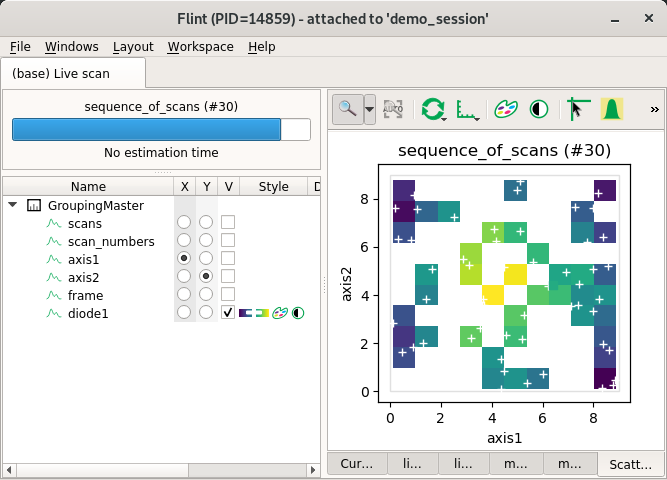
Non-regular scatters

Flint can display non regular scatters with solid rendering using 2D histogram.

This create a regular 2D mesh, and each cells can contain more than one value. The cell (the pixel) value is computed using a reduction function (for now it uses mean function).

Hint have to be provided to describe the size of the histogram grid. axis_points can not be specified because the axis is not regular. But axis_points_hint have to be used (with start and stop) and will be used to know the amount of pixels to used per axis.

start and stop have maybe no meaning here, so you can use min and max.

from bliss.scanning.scan_info import ScanInfo
import numpy

scan_info = ScanInfo()

# There is no hint for axis kind, and axis npoints is a hint
scan_info.set_channel_meta("axis1", group="foo", axis_id=0,
                           min=0, max=9, axis_points_hint=10, points=500)
scan_info.set_channel_meta("axis2", group="foo", axis_id=1,
                           min=0, max=9, axis_points_hint=10, points=500)
scan_info.set_channel_meta("diode1", group="foo")

# Request a specific scatter to be displayed
scan_info.add_scatter_plot(x="axis1", y="axis2", value="diode1")

# Generate the data
axis1 = numpy.random.rand(500) * 9
axis2 = numpy.random.rand(500) * 9
frame = numpy.mgrid[0:5, 0:100][0]
dist = (((axis1 - 4.5) ** 2 + (axis2 - 4.5) ** 2) ** 0.5)
dist = (dist.max() - dist) * 10
data = {
    "axis1": axis1,
    "axis2": axis2,
    "diode1": numpy.random.poisson(dist)
}

SCAN_DISPLAY.auto = True
simulate_scan(scan_info, data)

Non-regular 3D scatters

This also can work for extra dimensions with steppers.

from bliss.scanning.scan_info import ScanInfo
import numpy

scan_info = ScanInfo()

# There is no hint for axis kind, and axis npoints is a hint
scan_info.set_channel_meta("axis1", group="foo", axis_id=0,
                           min=0, max=9, axis_points_hint=10, points=500)
scan_info.set_channel_meta("axis2", group="foo", axis_id=1,
                           min=0, max=9, axis_points_hint=10, points=500)
scan_info.set_channel_meta("frame", group="foo", axis_id=2,
                           axis_kind="step",
                           start=0, stop=4, axis_points=5,
                           points=500)
scan_info.set_channel_meta("diode1", group="foo")

# Request a specific scatter to be displayed
scan_info.add_scatter_plot(x="axis1", y="axis2", value="diode1")

# Generate the data
axis1 = numpy.random.rand(500) * 9
axis2 = numpy.random.rand(500) * 9
frame = numpy.mgrid[0:5, 0:100][0]
dist = (((axis1 - 4.5) ** 2 + (axis2 - 4.5) ** 2) ** 0.5)
dist = (dist.max() - dist) * 10
data = {
    "axis1": axis1,
    "axis2": axis2,
    "frame": frame.flatten(),
    "diode1": numpy.random.poisson(dist)
}

SCAN_DISPLAY.auto = True
simulate_scan(scan_info, data)